PRAGMATRADING.COM1P R A G M A R E S E A R C H NOTE
TCA IS STRAI G H T F O R WA R D I N
THEORY BUT H A R D I N P R A C T I C E
The good practice of randomized trading experi-
ments is becoming more widely used, as seen
in the growing use of “wheels.” But traders still
face a big challenge when trying to decide which
of several different execution methods is better
because of a wide variety of confounding factors
and limited data set size available to most traders.
SO WHAT?
The risk is that traders make decisions based on
noise, and get worse outcomes for their investors.
This research note explores some real-world challenges,
and suggests best practices to develop confidence in
such comparisons given those challenges.
THE DATA SE T
To illustrate the challenges in a “controlled environ-
ment,” we work with a proprietary data set of 45,000
actual VWAP market orders traded in Q2-Q3 of 2020.
We use real orders because many of the challenges
in TCA result from the fat-tailed distribution of order
characteristics and performance results in real trading
data sets, and VWAP is a commonly used algorithm
by firms who quantitatively track execution shortfall.
VWAP SF NUM. OF
ORDERS
NOTIONAL
VALUE
SPREAD QTY /
ADV
AVG.
DURATION
1.26 bps 45,000 $24B 6.6 bps 0.8% 5 hours
TA B L E 1
Data summary with value-weighted performance.
NO. 25 | NOVEMBER 2 0 2 0
Measuring Execution Quality —
Finding the Signal in the Noise
A S I N G L E S I M U L AT E D
T R A D I N G E X P E R I M E N T
We simulate a typical trader’s “experiment.”
The trader has 400 parent orders per day to work
with, split across two algos, A and B, and reviews
performance after a 3 month period.
We simulate this experiment by choosing a random
3 month interval from our data set. To mimic a trader
splitting the day’s basket among algos, for each day in
the interval, we randomly assign each order to either
group A or group B with a coin toss. Of course, since
the same algo traded all the orders and the groups
were randomly assigned, groups A and B have the
same underlying performance. To simulate the situa-
tion where there are actually two different algos used,
one better than the other, we simply improve the
average price of each order in group A by 5% of
the spread, or about 0.3 bps on average. This creates
two different performance results, one for each algo.
Because we’re simply improving the average price
for the A group, we expect to improve its shortfall
regardless of what benchmark we decide to use.
The resulting data set for one such experiment
looks like this:
GROUP VWAP SF NUM. OF
ORDERS
NOTIONAL
VALUE
SPREAD QTY /
ADV
AVG.
DURATION
A –
Better
Algo
1.28 bps
(worse SF)
11,500 $6.4B 6.4 bps 0.86 % 5 hours
B –
Worse
Algo
1.21 bps
(better SF)
11,550 $6.9B 6.3 bps 0.88 % 5 hours
TABLE 2
Value-weighted performance summary of a single A/B experiment
over 3 months of data.
PRAGMATRADING.COM2N O V EM B E R 2 0 2 0
-20 -10 0 10 20
0
10
20
30
40
50
-2 -1 0 1 2
A looks better B looks better A looks better B looks better
0
25
50
75
100
125
C O U N T
S F D I F F E R E N C E ( B P S )
Arrival Price SF (bps) VWAP SF (bps)
SF DIFFERENCE (BPS)
Wrong
49%
Wrong
32%
TRUE PERFORMANCE BENEFIT OF A OVER B NO PERFORMANCE BENEFIT
F I G U R E 1
This figure shows a histogram of the difference between the average shortfall of algos A and B. Each point represents a single experiment
as described above, and the histogram shows the distribution of how often each outcome is seen when we repeat the experiment 500
times. Negative values mean that A was observed to be better than B (lower shortfall, the reality), 0 means they’re observed to be the
same, and positive means B was seen to be better than A.
In this particular experiment, algo B looks slightly
better—the opposite of the reality. After 3 months of
experiment, splitting flow cleanly across two algos, we
still got the wrong answer! But is this just an anomaly?
REPEATED RA N D O M S A M P L E S
Although in real life a trader only gets to see one
outcome of such an experiment, we can simulate the
random split of orders between two algos as many
times as we want, and we do so 500 times to get a
sense for how reliable such an experiment is. What
we’d hope is that we consistently see A outperforming
B, with perhaps a few anomalous cases where we got
the wrong answer. The histogram below shows each
such 3-month experiment as a single data point, and
the count of these outcomes bucketed by relative
outperformance of A over B (negative is good,
because lower shortfall). We illustrate the results both
in terms of VWAP shortfall and Arrival Price shortfall.
Note the “true” value (A is better than B by about
0.3 bps) is shown by the green line. We see that
for VWAP shortfall, the distribution of outcomes
is centered around that true value. Yet 1/3 of the
time, even this rigorously randomized 3-month
long experiment will give the wrong answer, shown
by the orange bars to the right of the dotted line,
and we’ll think that B is actually better than A.
Though for many traders Arrival Price slip-
page, shown in the left plot, is the true “gold
standard” performance metric, it’s a much
noisier metric.1 As we see below, measuring by
Arrival Price shortfall correctly identifies A as the
better algo only 51% of the time, barely more
than a random flip of a coin, and erroneously
crowns algo B as the winner 49% of the time!
1 For full-day orders, Arrival Price slippage varies by on
the order of the stock’s daily price change, since there is a
single point-in-time benchmark at the start, and trading occurs
throughout the day. In contrast, VWAP is effectively a rolling
average of prices calculated across the period of the trade,
so tends to deviate less from actual average price of an algo
that also spreads its trading out across the same period.
-20 -10 0 10 20
0
10
20
30
40
50
-2 -1 0 1 2
A looks better B looks better A looks better B looks better
0
25
50
75
100
125
C O U N T
S F D I F F E R E N C E ( B P S )
Arrival Price SF (bps) VWAP SF (bps)
SF DIFFERENCE (BPS)
Wrong
49%
Wrong
32%
TRUE PERFORMANCE BENEFIT OF A OVER B NO PERFORMANCE BENEFIT
F I G U R E 1
This figure shows a histogram of the difference between the average shortfall of algos A and B. Each point represents a single experiment
as described above, and the histogram shows the distribution of how often each outcome is seen when we repeat the experiment 500
times. Negative values mean that A was observed to be better than B (lower shortfall, the reality), 0 means they’re observed to be the
same, and positive means B was seen to be better than A.
In this particular experiment, algo B looks slightly
better—the opposite of the reality. After 3 months of
experiment, splitting flow cleanly across two algos, we
still got the wrong answer! But is this just an anomaly?
REPEATED RA N D O M S A M P L E S
Although in real life a trader only gets to see one
outcome of such an experiment, we can simulate the
random split of orders between two algos as many
times as we want, and we do so 500 times to get a
sense for how reliable such an experiment is. What
we’d hope is that we consistently see A outperforming
B, with perhaps a few anomalous cases where we got
the wrong answer. The histogram below shows each
such 3-month experiment as a single data point, and
the count of these outcomes bucketed by relative
outperformance of A over B (negative is good,
because lower shortfall). We illustrate the results both
in terms of VWAP shortfall and Arrival Price shortfall.
Note the “true” value (A is better than B by about
0.3 bps) is shown by the green line. We see that
for VWAP shortfall, the distribution of outcomes
is centered around that true value. Yet 1/3 of the
time, even this rigorously randomized 3-month
long experiment will give the wrong answer, shown
by the orange bars to the right of the dotted line,
and we’ll think that B is actually better than A.
Though for many traders Arrival Price slip-
page, shown in the left plot, is the true “gold
standard” performance metric, it’s a much
noisier metric.1 As we see below, measuring by
Arrival Price shortfall correctly identifies A as the
better algo only 51% of the time, barely more
than a random flip of a coin, and erroneously
crowns algo B as the winner 49% of the time!
1 For full-day orders, Arrival Price slippage varies by on
the order of the stock’s daily price change, since there is a
single point-in-time benchmark at the start, and trading occurs
throughout the day. In contrast, VWAP is effectively a rolling
average of prices calculated across the period of the trade,
so tends to deviate less from actual average price of an algo
that also spreads its trading out across the same period.
")